This project is designed and implemented as an extension of Yocto/GL, a collection of small C++17 libraries for building physically-based graphics algorithms. All credits of Yocto/GL to Fabio Pellacini and his team.
Introduction
As stated in the project title, we deal with volumetric path tracing (VPT) for heterogenous materials since it’s not currently supported by the actual release of Yocto/GL. In particular, we focus our implementation on heterogeneous materials, adding full support for volumetric textures and OpenVDB models. Next, we proceed with the implementation of delta tracking algorithm presented in PBRT book and two modern volumetric methods: spectral tracking from Kutz et al and unidirectional spectral MIS proposed by Miller et al.
Our work
OpenVDB support
The starting point of the project is to find a reliable and, of course, a working method to include OpenVDB data in Yocto. To do this we exploit data grids of the OpenVDB volumes and dump them using the official repo. A volume is made of voxels generically containing a float value that indicates the level of a property. In particular, we are dealing with density and, if present, temperature volumes.
To perform the conversion from .vdb to a Yocto-compatible format we start by looking at the grids the volume has using openvdb_print application. Usually, as said before, a volume contains a grid for the density and optionally one for the temperature. We dump these grids using a custom function and generating a .bin file for each of them. These files contain xyz coordinates of each voxel and the float value of the current property.
The format used for the Yocto-compatible files is .vol. We obtain these using yovdbload, which is a new application we implemented for volumes support that exploits yocto::image::save_volume(). In this part we find the bounding voxels coordinates of the volumes and, in case they are negative, translate them to have the lower bound in (0, 0, 0) and the max bound in (|min_x|+max_x, |min_y|+max_y, |min_z|+max_z), in which min and max are the smallest and biggest voxel coordinates.
Yocto/GL volumes add-ons
We introduce some changes in the original Yocto structure:
- New object properties in JSON files
- Volumes support in
yocto/yocto_sceneio.{h,cpp}andyocto_pathtrace/yocto_pathtrace.{h,cpp} - New options in
yscenetraceandysceneitracesapps - New
yovdbloadapp for volumes extraction - Insertion of
yocto_extension/yocto_extension.{h,cpp}with the implemented algorithms - Adapted path tracer routine in
yocto_pathtrace/yocto_pathtrace.{h,cpp}
Since we are dealing with a new type of objects, heterogenous volumes, we have to change a little bit the JSON features. We add a dedicated /volumes folder to store .vol files and a bunch of custom settings. Here is a list of the new properties that can be added to objects:
| JSON objects add-on | Type | Description |
|---|---|---|
density_vol |
.vol | Volume name containing density voxels |
emission_vol |
.vol | Volume name containing temperature voxels |
scale_vol |
vec3f | XYZ scale of the volume |
offset_vol |
vec3f | XYZ center offset of the volume |
density_mult |
float | Handles the level of density of the volume |
radiance_mult |
float | Handles the level of radiance the volume emits |
All those features are then handled by yocto::sceneio and yocto::pathtrace that we change accurately. After adding also volumes support to the rendering apps yscenetrace and ysceneitraces, we introduce a new option for the execution permitting us to choose one of the volumetric path tracing algorithms: --vpt,-v {delta, spectraltracking, spectralMIS}.
Concerning the algorithms, yocto::extension contains all the needed functions. Here is a listing:
| Function | Description |
|---|---|
check_bounds() |
Checks if XYZ indices are inside the bounds |
gen_volumetric() |
Fills a volume with a volumetric texture using Perlin noise |
has_vpt_volume() |
Checks if an object is a heterogenous volume |
has_vpt_density() |
Checks if a volume has density voxels |
has_vpt_emission() |
Checks if a volume has temperature voxels |
eval_vpt_density() |
Evaluates the density value at the given real coordinates |
eval_vpt_emission() |
Evaluates the temperature value at the given real coordinates |
eval_delta_tracking() |
Implementation of delta tracking algorithm |
eval_spectral_tracking() |
Implementation of spectral tracking algorithm |
eval_unidirectional_spectral_mis() |
Implementation of unidirectional spectral MIS algorithm |
We use those methods to compute all the necessary parameters like the density in a ray intersection point or the path tracing in volumes using different techniques. In particular, volumes are implemented using yocto::image::volume structure and other functions from the same namespace like yocto::image::eval_volume() which evaluates a voxel value at given coordinates. Further details on the methods implemented here.
The structure for the vsdf is changed as following:
  struct vsdf {
    vec3f density    = {0, 0, 0};
    vec3f scatter    = {0, 0, 0};
    float anisotropy = 0;
    bool  htvolume   = false;
    vec3f scale = {1.0, 1.0, 1.0};
    int event = 0;
    const trace::object* object = nullptr;
  };
It now contains heterogeneous volume flag for the path trace, a scale for voxels evaluation, the type of event happening and the object to which it refers to retrieve other information. The events are divided in {EVENT_NULL, EVENT_SCATTER, EVENT_ABSORB} and permits us to track the current situation of the rays path. The first one stands for the case when a null collision happened and means that a fictitious particle has been hit. We remind that in null-scattering algorithms we can see a heterogeneous volume as a mixture of real and fictitious particles and proceed on a path direction if these latter have been hit. The second event refers to the scattering case when a real particle has been hit and we have to scatter the ray. Finally, EVENT_ABSORB is the case when there is an absorption of the ray which leads to its extinction.
The structure of the path tracer in yocto::pathtrace has undergone some changes to deal with the three different volumetric algorithms. A parameter std::string vpt is added to the trace_params structure in order to know the type of tracing. This value is automatically linked with the rendering app. The flow of the trace is a little different from Yocto’s one because of a different approach used. In fact, we compute the weights and the distances of the three volumetric algorithms inside the functions themself instead of taking a step-by-step approach in the main pathtrace. The weights are then multiplied by the main weight of the current trace. This new approach, which “forecasts” the total interaction in a single function step (that is O(n) with n the number of sampled distances) and which is also recommended by our references, shows a nice speedup on the computation of the paths. We also decide to compute the transmittance along the path in a simultaneous way instead of performing another cycle which would lead to O(n2). This further change scores a remarkable speedup of about 2x.
Delta Tracking
The first algorithm we focus on, and the classic one if we want to say, is delta tracking. This algorithm, like the next two we are going to implement, is interpreted as filling the medium of real particles with additional particles, the fictitious ones. This leads to a study based on whenever a real particle has been hit and how the ray should behave. Moreover, we extend the basic version of delta tracking from PBRT, which handles only scattering and null collision events, with the modified version from Kutz et al. This permits us to make a comparison of similarities and computational times with the next two techniques in the Results section. In this algorithm, the spectrum of the scatter is the treated taking the majorant of the channel without considering the others. We will see in the spectral MIS section why this choice has a big impact on the algorithm performances.
The mixed version of delta tracking we implement, and that produced the best results along the others, can be resumed as follow:
- Sample a distance t. If t is greater than the maximum distance, i.e. the edge of the volume, exit.
EVENT_ABSORB: Exit with weight=1 and evaluate the emission of the volume.EVENT_SCATTER: Exit with weight=T*s and sample incoming direction with the sample phase function.EVENT_NULL: If the precedent events don’t occur, continue.
in which T is the trasmittance computed simultaneously and s is the scatter. This is just a simple list of steps of what’s happening; refer to extension for further details.
Spectral Tracking
Another implemented approach follows the Spectral Tracking algorithm proposed by Kutz et al. Each interaction with the volume is now resolved across all the defined spectrum (in our case the 3-channels RGB spectrum). We decided to implement Spectral Tracking in order to compare differences between Delta tracking, and the next algorithm that will be proposed, namely Spectral MIS.
Further details on the implementation here.
Unidirectional Spectral MIS
The novelty introduced by the unidirectional spectral MIS in respect of the precedent algorithms is that it doesn’t deal only with the majorant of the scatter but samples a different channel each times, considerably reducing the computing times. For example, if we assume to have a 3-channel (RGB) non-uniform scatter with an high value on the green channel and lower ones on the other, the spectral MIS performs with a much lower computational time w.r.t. delta tracking and spectral tracking. In fact, here the spectrum is handled using each of the present channels. The speedup of this algorithm borns from the fact that instead of considering the majorant of the spectrum we consider a random channel of it and this leads to have bigger sampled distances when the value of the channel is small. Of course, the bigger sampled distances are, the smaller are the steps inside the volume. This technique is really useful for a faster convergence. However, we notice to have problems with this method and decide to use the mean of the spectrum values, which remains a faster technique than the one used in the precedent algorithms.
We can resume spectral mis these salient steps:
- Tracking of path contributions and pdfs (f,p).
- Compute the mean of the scatter and multiply it by the max density to have a weighted majorant.
- Sample a distance t using the weighted majorant. If t is greater than the maximum distance, i.e. the edge of the volume, exit.
- Compute sigma_t, sigma_s, sigma_a, sigma_n.
- Sample an event e using sample_event() and the probabilities of each event normalized with the max density.
EVENT_ABSORBorEVENT_SCATTER: Exit with updated weight and evaluate the emission of the volume.EVENT_NULL: continue.
Another important term here is the sample_event() function which, in our implementation, is based on this thread. The probabilities we use for this function are computed using the sampled channel of sigma_a, sigma_s and sigma_n, normalized with the max density. Then we add to the path contribution f a different value which depends on the sorted event and the trasmittance T if absorption or scattering occur. Absorption and scattering are treated in the same way in the main loop but, like for the other two algorithms, we compute the emission in the first and sample the incoming direction with the phase function in the second. Another simplification is that the path of pdfs is equal to the one of contributions using the cancellation trick. At the end, if absorption or scattering occur, we return a weight which is made of the path of contributions divided by the mean of p. Refer to extension for further details.
Results
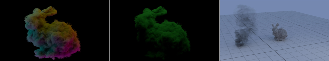
In order to compare the proposed algorithms, we propose three scenarios on which heterogeneous volumes are evaluated:
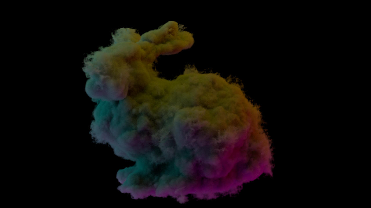
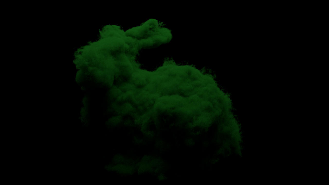
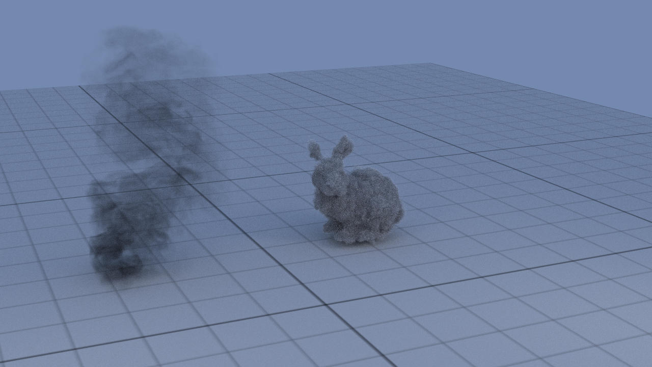
- Homogeneous Albedo: bunny cloud exposed to 4 large light panels on left/right, up/down sides. Each panel emits a different light. The cloud material has an uniform albedo vector, hence it uniformly scatters all the colors.
- Heterogeneous Albedo: Same setup of H.A. scene, but only the upper panel is lit, and it emits white light. The cloud material has an heterogeneous albedo; green channel is fully scattered while RB spectrum is fully absorbed.
- Scene 3: Simple scene with smoke2 and bunny_cloud densities from OpenVDB.
For each scene, each algorithm was executed with 3 different sampling quality, namely:
- 16 spp
- 256 spp
- 2048 spp
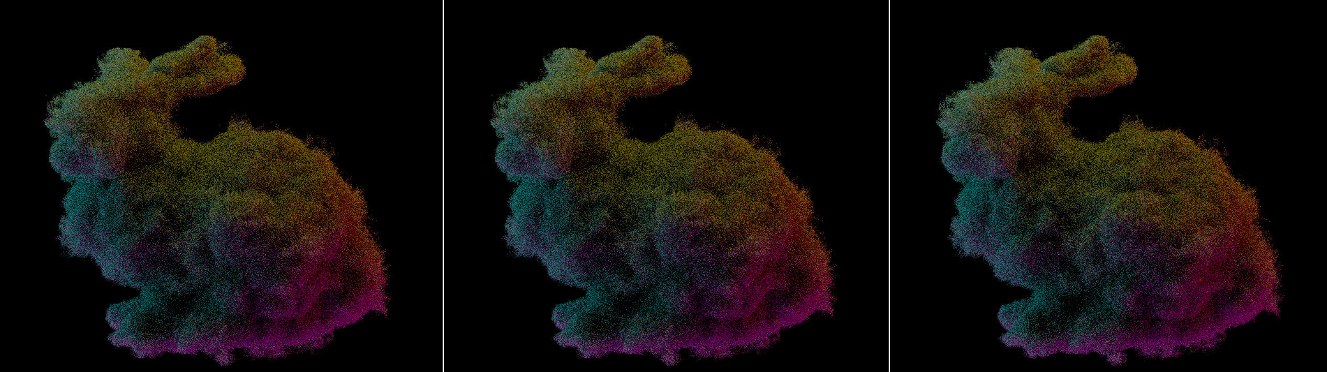
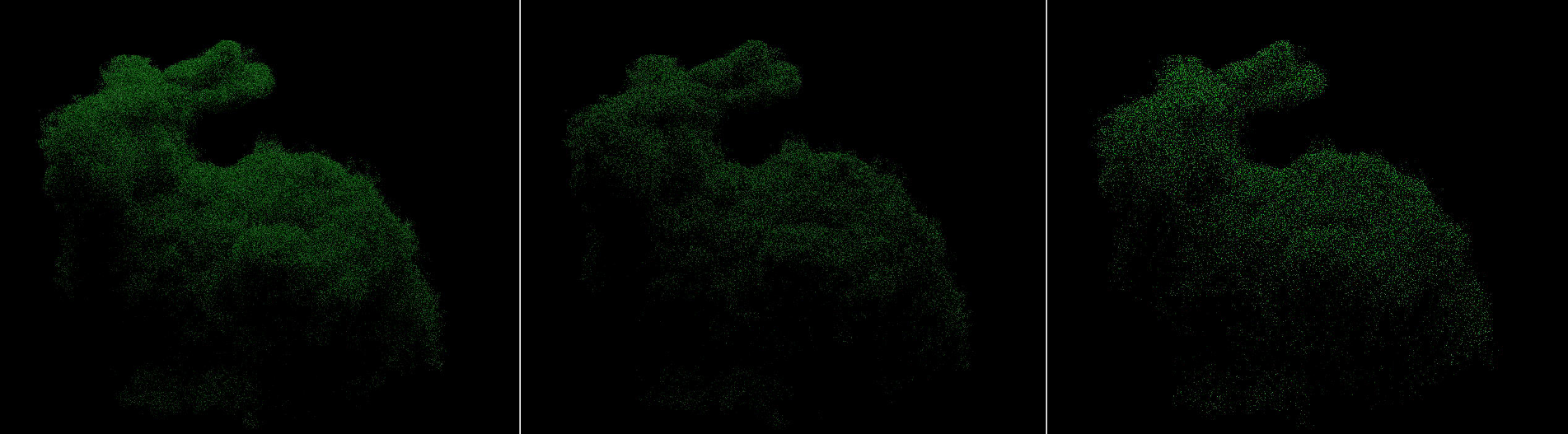
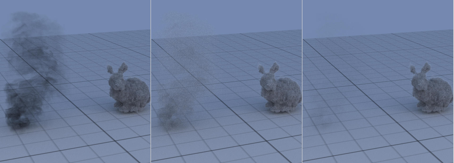
In the following section, comparison images will be shown. Each image is divided into 3 frames, from left to right they are:
- Delta Tracking
- Spectral Tracking
- Spectral MIS
Homogeneous Albedo
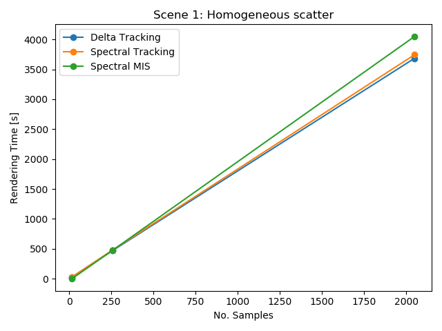
 Regarding the first scene, it is possible to notice how already with 16 spp, all the algorithms approaches convergence. As expected from the theory, no peculiar performance difference can be noticed between DT, ST and SMIS. We also provide a comparison of the result at 16 spp, plus a plot showing rendering timings for the scene wrt No. of samples:
Heterogeneous Albedo
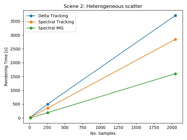
 For the second scene, we expected a wider difference between rendering times between DT, ST and SMIS, since the last algorithm relies on the same heterogeneity of the spectrum extintion in order to quickly estimate volume collisions. We noticed almost a 2x speedup during the renderings of this scene while using SMIS.
Scene 3
 In the last scene we wanted to understand how clouds behaved with objects, namely the floor. It’s quite interesting to see how clouds project shadows onto the floor. Regarding the comparison, the 3 methods gave quite different results. We do not report the timing plot for this scene since the results are similar to H.S. scene.
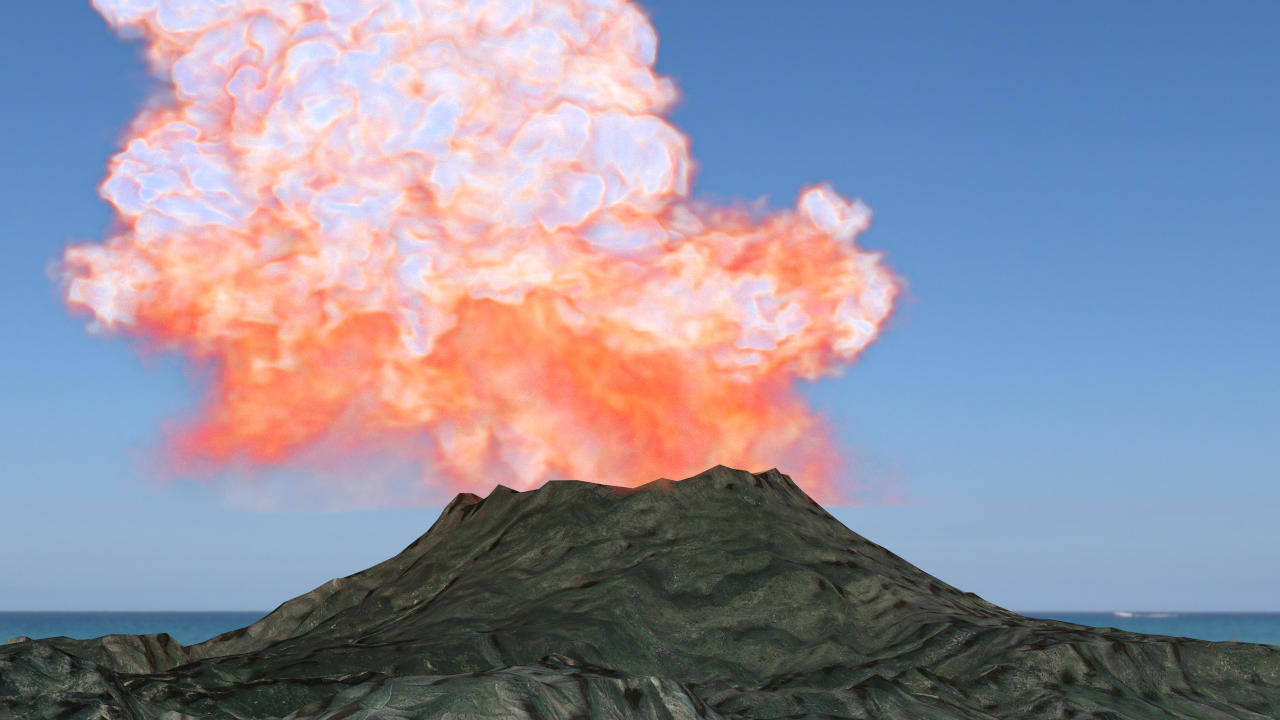
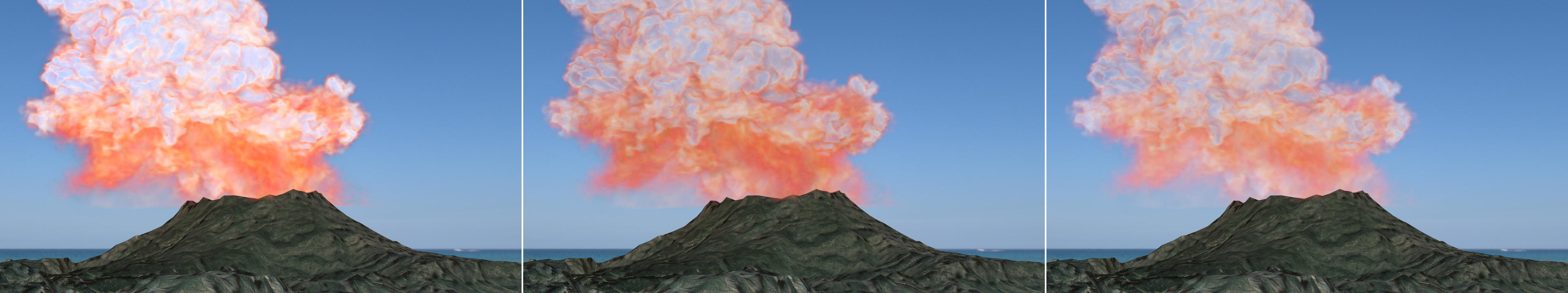
Full testing scenes
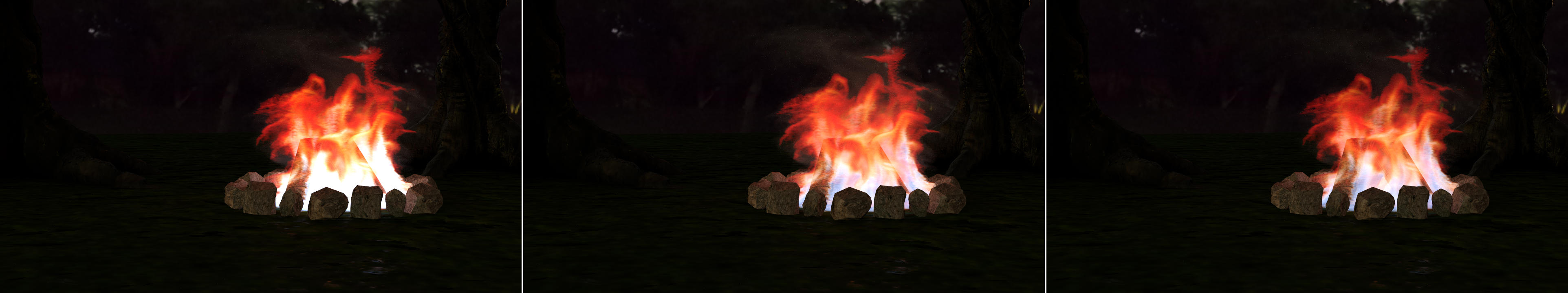
Here we propose some of our testing scenes with a comparison of the three algorithms, disposed in the same way as before (Delta Tracking - Spectral Tracking - Spectral MIS). It’s possible to notice that when the temperature comes in, the three algorithms differs a bit on the emitted radiance. Instead, as shown in the image of the modified Disney cloud, when there’s no emission the outputs look identical.
![]()


Installation and usage
To use this extension make sure you own all the requirements from Yocto/GL.
Now simply clone/download the repo and follow these steps:
cd yocto-gl-vptsh scripts/build.shsh scripts/run.sh
In this repo we provide a standard scene of homogeneous volumes from Yocto/GL. If you wish to try out the scenes showed before with heterogeneous volumes you can download them here. Unzip the package you downloaded and put it in the /tests folder. Now you should edit /scripts/run.sh and add a line for the scene you want to render, e.g.:
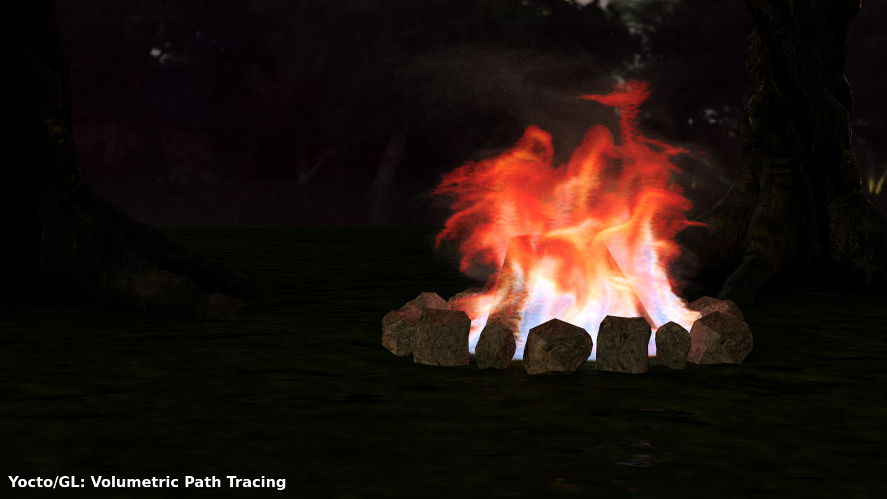
./bin/yscenetrace tests/campfire/campfire.json -o out/lowres/campfire.jpg -t path -s 4096 -r 1280 -v delta
which uses yscenetrace app to render the scene, from the campfire json, using the pathtrace (-t), with 4096 samples (-s), resolution of 1280 (-r) and using delta tracking algorithm (-v).
Credits
References
- Yocto/GL
- Spectral and Decomposition Tracking for Rendering HeterogeneousVolumes, Kutz, Peter & Habel, Ralf & Li, Yining & Novák, Jan.
- A null-scattering path integral formulation of light transport, Miller, Bailey and Georgiev, Iliyan and Jarosz, Wojciech
- Physically Based Rendering: from Theory to Implementation
- Production Volume Rendering, Pixar Animation Studios
- OpenVDB
- Disney clouds